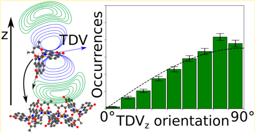
Tuning the orientation of the transition dipoles of emitter molecules in organic layers for optimal outcoupling efficiency is an essential ingredient towards 100% quantum efficiency of OLED devices. The molecular orientation of emitters is determined by the interaction with their host materials. Here, we present a systematic study of the impact of functional side groups of emitter molecules on the alignment of their transition dipoles (TD) in a CBP host. Furthermore, we illustrate how virtual experiments can aid the design of emitter molecules.
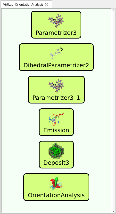
The workflow, as predefined in the trial version of our virtual lab (available here), is illustrated in the figure to the right and follows simulation steps below. In the pre-defined workflows, you can see and modify the settings (e.g. input files) of each module by double clicking on the icon.
- Computing forcefield-parameters for CBP (modules labeled Parametrizer3 & DihedralParametrizer2 in the workflow):
As input for the Parametrizer you can use a pre-optimized 3D structure either generated with our “synthesis” equivalent tool in the mol2 format, or use the input cbp.mol2 provided in the trial version. The Parametrizer generates two relevant files: molecule.pdb and molecule.spf. Load molecule.pdb and molecule.spf in the DihedralParametrizer module to generate customized energy profiles for rotation of flexible side groups of your molecule. - Computing forcefield-parameters for the emitter molecule:
Similar for CBP, load the input (either the mol2 files provided or generated with our “synthesis” tool) of one of the emitter molecules in the Parametrizer3_1 module. Therefore, we provide as an example Ir(bppo)2acac, Ir(bppo)2(ppy) or Ir(bppo)(ppy)2 as mol2-files here. - The Emission module computes transition dipole of the emitter molecule. Therefore, select the optimized molecule output from the Parametrization, namely Parametrizer3_1/molecule.pdb using the drop down menu next to the input-file field. Set Emission type to Phosphorescent and enable “Orientation Analysis Output” and provide ids of three atoms that generate three linearly independent vectors with the center of the molecule. As an example, for Ir(bppo)(ppy)2 the three N-atoms can be used (1, 27 and 54). Select the center of the molecule manually or check the Automatic Center Atom box (select 0, corresponding to the Ir-atom, for the Ir-Emitter molecules). You can imagine that three vectors are constructed out of the three coordinates of the Ir-atom and the coordinates of each N-atom. For the Ir(bppo)2acac, you can use one of the N-atoms of the bppo groups (17 or 18) and two C-atom of the acac-group, which are connected to the Ir-atom.
- Then, you can use Deposit, to generate a thin film of 1200 molecules and a box of Lx=40, Ly=40, Lz=120 (in Angstrom). Note that these parameters define half the box size each, so the resulting morphology will extend from -40 A to +40 A in x and y-direction. Make sure that the Final Temperature is set to 300 K, Number of Steps is 130000, Number of SA cycles is 32 and Dihedral Moves is checked. As input for Deposit (Molecules tab), provide the CPB input (molecule.pdb from the Parametrizer3 module and the dihedral_forcefield.spf from the DihedralParametrizer2 module) at a concentration of 0.9, i.e. 90%, and the Emitter input (molecule.pdb and molecule.spf from the Parametrizer3_1 module) at 0.1, i.e. 10%. Make sure not to confuse the inputs, i.e. note the difference between Parametrizer3/molecule.pdb (CBP) and Parametrizer3_1/molecule.pdb (Emitter). Keep the Extend morphology (x,y) checked in the last tab (Postprocessing).
- In the Orientation Analysis module, provide the output of the Deposit-Morphology (Deposit3/structure.cml), enable TD Analysis and provide the file Emission/orientation_analysis_input.yml containing information of the transition dipoles computed in step 3. Disable Axes Analysis.
All settings not explicitly mentioned above should be kept as set in the pre-defined workflows. For details on the individual settings, check out our documentation page or write as at info.nanomatch.com. Details on the morphology generation are available here. Note that you do not need to wait for each simulation step to finish for file transfer to the next module: You can define the data-transfer between modules using the dropdown menues next to the respective file-input fields before submitting the full workflow. See the predefined workflows in the trial or this webinar for reference.
A note on resources: Parametrizer, DihedralParametrizer, Emission and Deposit scale well for up to 32 cores. We recommend to allocate 32 cores, if available, using the Resources Tab in the GUI. The Orientation analysis can be done on a single core.
Once the workflow is defined as described above, connect to your computational resource using the “Connect” button (top right in the GUI) and press Ctrl+R or “Run->run” in SimStack. Now, all you need to do is to wait for the simulation to finish.
Results:
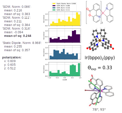
At first, the results of the Emission will deliver you an impression of the calculated molecule and its TD vectors, their absolute orientation with respect to the molecule and relative norms to each other, determined by the length of the vectors. A file, named dipole_and_phosphorescence.tcl can be visualized using e.g. VMD, will present this, which is also done in the figure below. In this figure, Ir(bppo)2acac and the three TD (golden arrows) of this molecule and its static dipole (red arrow) are illustrated.
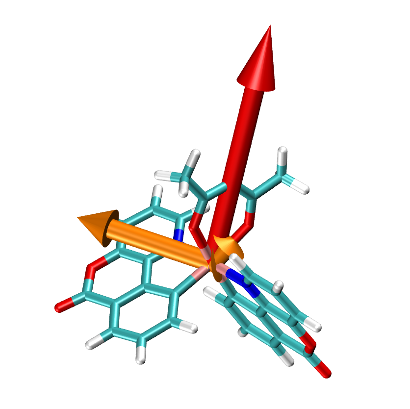
Generally, phosphorescent molecules have three TD, abbreviated as ‘SOM’, corresponding to second order moments. The molecule oscillates along the SOM, enabling the emission of the phosphorescent light. For Ir(bppo)2acac two of the three SOM are really small. The norm of SOM is proportional to the life time of the phosphorescent light, emitted in the plane, which is orthogonal to this vector.
In the following, the SOM are used in the TD-Analysis. Thus,vectors, having a large norm, are more relevant for the further analysis. We use them to predict the an- or isotropy of the emitters, which is expressed in terms of an orientation descriptor. An orientation descriptor 1/3 or larger corresponds to an totally isotropic orientation, and on the contrary lower values than 1/3 to a preferential in-plane orientation.
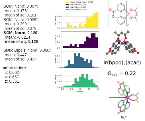
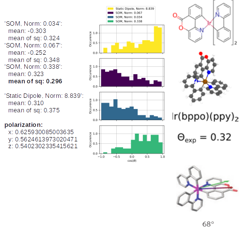
The TD-Analysis delivers a file orientation_analysis.yml and png file, which can be used to distinguish the orientation of the emitters in the host material. The picture below shows at the these results at the left side: the norm of the SOM and the mean of the corresponding orientation descriptor are presented. The orientation descriptor of the different SOM distributions for all emitters, embedded in the morphology, are presented in the histograms. The right part of the figure is taken from Ref[1,2], in which the same approach was used to predict the anisotropy of those Ir-emitter molecules (Ref[1]) and compared to experimental values (Ref.[2]). In experiments a combination of the three SOM is detected, which is also displayed in the figure as green arrow, which fits quite well with the SOM, having the largest norm of our Emission-prediction, which was presented with the golden arrow in the previous picture.
 |
Taken together, we present a analysis to measure the the an -or isotropy of emitters embedded in host materials, created by our Deposit module. Thus, the TD-Analysis, using the results of the Emission, can be used to study a potential orientation of new emitters or the effect of the host material.
Ir(bppy)2(acac): the SOM with the highest norm (0.120) corresponds to the blue histogram and a corresponding orientation descriptor of 0.126. The experimental value of 0.22 is slightly higher, nevertheless, it demonstrates that the emitter orientation is treated correctly as an isotropic emitter. In the mentioned previous study, the analysis of Ref. [1] predicted an orientation descriptor of 0.19. The different morphologies cause those slightly different values, however, the same physical properties of the emitter is predicted. The last three below the SOM analysis correspond to the phosphorescent emission in the x, y, z-axes, which can be compared relatively. This also clearly shows that there is a preferred orientation of Ir(bppy)2(acac) in CBP.
The same analysis for Ir(bppo)2(ppy) and Ir(bppo)(ppy)2 below, shows that the direct comparison between the previously introduced Ir(bppy)2acac shows the right reproduction of the an- or isotropy of the emitters. Especially, the polarization introduces directly with an obvious interpretation that Ir(bppo)2(ppy) and Ir(bppo)(ppy)2 are emitting in all axes with a similar intensity, however, Ir(bppy)2(acac) showed a much lower emission along the z-axis
 |
 |
Taken together, this experiment introduced a Workflow in which a combined morphology of host and emitter molecules can be created and analyses. In a next step, you can try to change the host or emitters with other molecules of your interest and rerun the whole study, rising your knowledge of the selected materials.
[1] P. Friederich et al. Chem. Mater. 2017, 29, 9528-9535
[2] M. Jurow et al. , Nat. Mater. 2016, 15 (1), 85−91.